Using Taylor Series

\[ f(x) = f(0) + \frac{f^\prime(0)}{1!}x + \cdots + \frac{f^{(n-1)}(0)}{(n-1)!} x^{n-1} + \frac{f^{(n)}(0)}{n!} x^{n} = f(0) + \sum_{k=1}^n \frac{f^{(k)}(0)}{k!} x^k\,,\]

As a refresher, I'll write out the Taylor series expansion of \(\sin(x)\) with four terms to showcase how it works.

f(x) = sin(x)
f′(x) = cos(x)
f″(x) = -sin(x)
f‴(x) = -cos(x)

taylorsin(x) = f(0) + f′(0)/factorial(1) * x + 
               f″(0)/factorial(2) * x^2 + 
               f‴(0)/factorial(3) * x^3

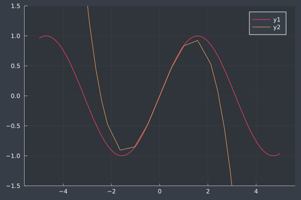
plot(f)
plot!(taylorsin, ylim=(-1.5, 1.5))

It's clear from the plot that from \(-1 \leq x \leq 1\), our polynomial expansion is a really good approximation of the \(\sin(x)\) function. More terms will improve the approximation for a larger interval.

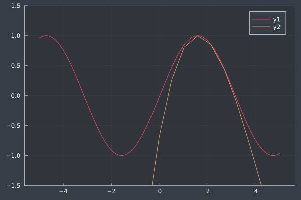
While the above plot shows approximating about the origin, we can also approximate about other points. We'll write out the expansion approximating the point \(a\). Instead of all of our evaluations at \(f(0)\), we'll evaluate at \(f(a)\). And instead of \((x-0) = x\) for the \(x\) components, we'll use \((x - a)^j\). Therefore, when \(x = a\), the term goes to zero like before. Suppose \(a = 2\).

a = 2

taylorsin(x) = f(a) + f′(a)/factorial(1) * (x - a) + 
               f″(a)/factorial(2) * (x - a)^2 + 
               f‴(a)/factorial(3) * (x - a)^3

plot(f)
plot!(taylorsin, ylim=(-1.5, 1.5))