Using Sigmoid Functions
The sigmoid function is defined as,
\[ S(x) = \frac{1}{1 + \exp(-kx)} \,,\]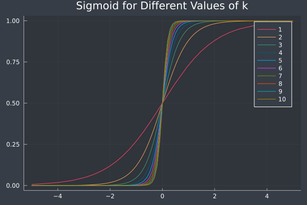
and creates an "S" shape when plotted which ranges from \(0\) to \(1\). As we vary \(k\), we see that the slope increases.
\(k\) is sometimes called the gain.
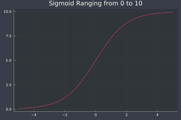
Therefore \(S(x)\) is often used to normalize values in \(\mathbb{R}\) to \(\mathbb{R}^{[0, 1]}\). A variation of \(S(x)\) is where we can scale the sigmoid to \(\mathbb{R}^{[0, \mu]}\),
\[ S_\mu(x) = \frac{\mu}{1 + \exp(-kx)}\,.\]Let \(\mu = 10\) and \(k = 1\), then \(S_\mu(x)\) yields the plot below.
You likely already see the power of this function as it has a domain over the reals from \(-\infty\) to \(\infty\) and is bijective with a codomain over the reals from \(0\) to \(1\). Furthermore, as we have seen, varying \(k\) will impact the slope of the function.
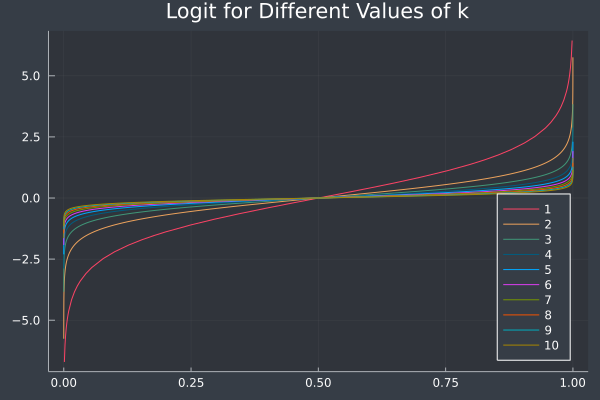
In a finite environment, \(S(x)\) may appear to be surjective, but it indeed is bijective and has an inverse – the Logit function,
\[ S^{-1}(x) = \frac{1}{k}\log\Big( \frac{x}{1-x} \Big) = \frac{1}{k}\Big( \log(x) - \log(1 - x)\Big)\]