Riemann Sums

The core operations of the Calculus are "infinite subtraction" (or differentiation) and "infinite summation" (or integration). In the latter realm, we can leverage a discretized version which uses Riemann Sums.

When it comes to a bunch of basic shapes like rectangles, circles, and triangles, we have simple formulas to compute their areas.

We know that for a rectangle with sides of length \(a\) and \(b\), the area is just the product \(a\cdot b\), for circles it's \(\pi r^2\) and triangles use \(\frac{1}{2} b\cdot h\).

The Riemann sum is defined as,

\[ S = \sum_{i=a}^b f(x_i^\star) \Delta x_i \]

where \(\Delta x = \frac{b - a}{n}\) and \(x_i^\star\).

The fundamental idea here is that in order to find the area under the curve, \(f(x)\), we look at the interval \(a \leq x \leq b\) and break it into \(n\) partitions.

Suppose we have the function \(f(x) = x^2\) and we want to compute the area between interval \(0\) and \(3\). We choose to use \(n\) partitions where \(n = 3\).

We then can compute the partition or step-size,

\[ \Delta x = \frac{b-a}{n} = \frac{3 - 0}{3} = 1 \,,\]

yielding the intervals \(\{ (0, 1), (1, 2), (2, 3) \}\).

Writing out the terms of \((1)\), we get,

\[\begin{aligned} S &= f(0)\cdot 1 + f(0 + 1) \cdot 1 + f(0 + 2\cdot 1) \cdot 1 + f(3)\cdot 1 \\ &= f(0) + f(1) + f(2) + f(3) \\ &= 0 + 1 + 4 + 9 \\ &= 14 \end{aligned}\]

Let's write out how we compute this in Julia.

function riemann(f::Function, a::Int, b::Int, n::Int)
    Δx = (b - a)/n
    s = 0
    for (k, x) in enumerate(a:Δx:b)
        s += f(x)*Δx
    end
    return s
end

The integral \(\int_0^3 f(x)\ dx = \frac{1}{3}x^3\ \Big\vert_0^3 = \frac{1}{3}\Big( 3^3 - 0^3 \Big) = 9\).

As we increase the number of partitions, the result becomes increasingly more accurate.

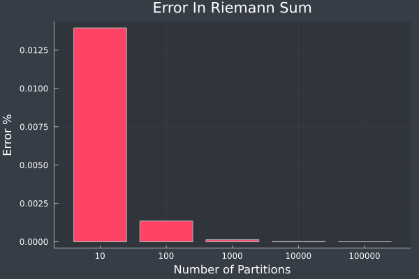
This should make sense since the integral is defined as when the number of partitions approaches infinity.