Representing Graphs

Graphs consist of nodes (or vertices) connected by edges. If the edges are bi-directional, then we just call it a graph. If the edges have direction, then we call it a directed graph or sometimes a digraph. If the edges have values (or weights) associated with them, then we call it a weighted graph or weighted digraph. Finally, a graph can be cyclic if it's both directed and at least one node contains a path back to itself. If it doesn't posess that "link back" property, then it's called acyclic.

In mathematical notation, we express a graph, \(G\), with a tuple which notes the number of vertices and edges,

\[ G = (V, E)\,. \]

Below is an example of simple graph. There are no weights or directions between nodes. Because there are no directions, we don't speak of it being cyclic.

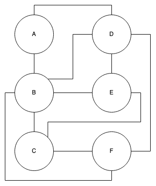Figure 1: Simple Graph

While in the next example, we can see a cyclic graph because each edge is uni-directional and we can see that multiple nodes have paths which cycle back, e.g. \(A \rightarrow B \rightarrow D \rightarrow A\) and \(B \rightarrow C \rightarrow F \rightarrow B\).

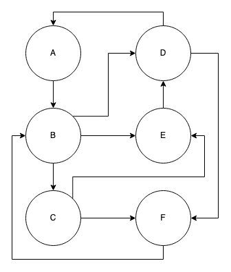Figure 2: (Cyclic) Directed Graph

Different Ways to Represent Graphs

In computer science, there are several ways which we can represent graphs, the most common being incidence matrices, adjacency matrices, edge lists, and adjacency lists. Choosing a representation will depend on the types of operations a specific project will be applying most frequently as there are pros and cons to each implementation.

Incidence Matrices

WIth an incidence matrix, the rows represent vertices, \(V\), and the columns represent edges, \(E\), yielding a \(V \times E\) bit-matrix. Therefore, if we were to represent the simple matrix in figure 1, it would be a \(6 \times 10\) matrix.To apply indexing to the edges, we first need to label them.

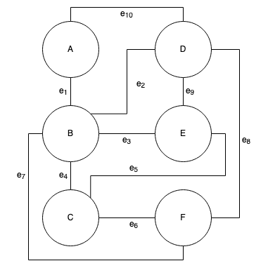Figure 3: (Cyclic) Directed Graph with Labeled Edges
\[ \begin{bmatrix} & e_1 & e_2 & e_3 & e_4 & e_5 & e_6 & e_7 & e_8 & e_9 & e_{10}\\ A & 1 & 0 & 0 & 0 & 0 & 0 & 0 & 0 & 0 & 1 \\ B & 1 & 1 & 1 & 1 & 0 & 0 & 1 & 0 & 0 & 0 \\ C & 0 & 0 & 0 & 1 & 1 & 1 & 0 & 0 & 0 & 0 \\ D & 0 & 1 & 0 & 0 & 0 & 0 & 0 & 1 & 1 & 1 \\ E & 0 & 0 & 1 & 0 & 1 & 0 & 0 & 0 & 1 & 0 \\ F & 0 & 0 & 0 & 0 & 0 & 1 & 1 & 1 & 0 & 0 \\ \end{bmatrix} \]

incmat = [
    1 0 0 0 0 0 0 0 0 1 ;
    1 1 1 1 0 0 1 0 0 0 ;
    0 0 0 1 1 1 0 0 0 0 ;
    0 1 0 0 0 0 0 1 1 1 ;
    0 0 1 0 1 0 0 0 1 0 ;
    0 0 0 0 0 1 1 1 0 0 ]

Adjacency Matrices

With an adjacency matrix the rows and columns both represent the nodes, where a \(1\) in the \(a_{ij}\) position represents a connection from \(i\) to \(j\). Therefore for our simple graph where edges have no direction between nodes,

\[\begin{bmatrix} & A & B & C & D & E & F \\ A & 0 & 1 & 0 & 1 & 0 & 0 \\ B & 1 & 0 & 1 & 1 & 1 & 1 \\ C & 0 & 1 & 0 & 0 & 1 & 1 \\ D & 1 & 1 & 0 & 0 & 1 & 1 \\ E & 0 & 1 & 1 & 1 & 0 & 0 \\ F & 0 & 1 & 1 & 1 & 0 & 0 \\ \end{bmatrix}\,.\]

Notice that the matrix is symmetric. Compare this to an adjacency matrix for the directed graph version where there is direction, remember that a \(1\) in the \(a_{ij}\) component means that a connection maps from \(i\) to \(j\).

\[\begin{bmatrix} & A & B & C & D & E & F \\ A & 0 & 1 & 0 & 0 & 0 & 0 \\ B & 0 & 0 & 1 & 1 & 1 & 1 \\ C & 0 & 0 & 0 & 0 & 1 & 1 \\ D & 1 & 0 & 0 & 0 & 0 & 1 \\ E & 0 & 0 & 0 & 1 & 0 & 0 \\ F & 0 & 1 & 0 & 0 & 0 & 0 \\ \end{bmatrix}\]

Edge Lists

With edge lists, we simply maintain an array of tuples, each as \((i, j)\).

edgelist = [   
    (a, b), (b, c), 
    (b, d), (b, e), 
    (c, e), (c, f),
    (d, a), (d, f), 
    (e, d), (f, b)]
@show edgelist
> edgelist = [(1, 2), (2, 3), (2, 4), (2, 5), 
>             (3, 5), (3, 6), (4, 1), (4, 6), 
>             (5, 4), (6, 2)]

Adjacency Lists

With adjacency lists, for a graph with \(|V|\) vertices, there is an array with \(|V|\) elements where each element represents a vertex. For each vertex, there is an array of all its connections, or edges.

adjacencylist = [
    [b, d],
    [a, c, d, e, f],
    [b, e, f],
    [a, b, e, f],
    [b, c, d],
    [b, c, d]]
@show adjacencylist
> adjacencylist = [[2, 4], [1, 3, 4, 5, 6], 
>                  [2, 5, 6], [1, 2, 5, 6], 
>                  [2, 3, 4], [2, 3, 4]]