Norms

Norms are a generalization of a length function and ultimately are used for computing the length of vectors in an abstract vector space.

Let \(V\) be an abstract vector space over a field \(\mathbb{F}\). The norm is a function, \(\eta : V \rightarrow \mathbb{R}\) such that,

1. \(\eta(x + y) \leq \eta(x) + \eta(y)\) for all \(x, y\) in \(V\).

2. \(\eta(\alpha x) = \vert \alpha \vert \eta(x)\) for all \(x\) in \(V\) and \(\alpha\) in \(\mathbb{F}\).

3. For all \(x\) in \(V\), \(\eta(x) = 0\) if and only if \(x = 0\).

For each of the following norms I discuss below, I've provided an implementation in Julia. That being said, there's a great package Distances which includes all of these and more. While my implementations are good for solidifying the concepts behind the individual functions, they are likely not as efficient as those defined in Distances.

Absolute Value Norm

The absolute value function,

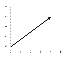
\[ \eta(x) = \vert x \vert\,. \]

In \(1\)-dimensional space, the vector which extends from the origin to \(\pm x\) has a length of \(x\).

The vector \(\pm 4\) has a length of \(4\).

\(\ell^1\) Norm

The \(\ell^1\) norm will trace along the individual components of a vector rather than calculate the distance along the hypotenuse,

\[ \eta(x) = \sum_{i=1}^n \vert x_i \vert \,.\]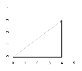

Therefore, by the \(\ell^1\) norm, the \((4, 3)\) vector has a length of \(4 + 3 = 7\).

l1_norm(X) = [abs(x) for x in X] |> sum

l1_norm([4 ; 3])
> 7

\(\ell^2\) Norm

The \(\ell^2\) norm is for computing the length of a vector in \(n\)-dimensional space, defined as,

\[ \eta(x) = \lVert \mathbf{x} \rVert = \sqrt{x_1^2 + \cdots + x_n^2 }\,. \]

Notice that this is the same as the square root of the inner product of a vector with itself, \(\sqrt{\mathbf{x}\boldsymbol{\cdot} \mathbf{x}}\).

By the \(\ell^2\) norm, the vector \((4, 3)\) has a length of \(\sqrt{3^2 + 4^2} = \sqrt{9 + 16} = \sqrt{25} = 5\).

l2_norm(X) = [x*x for x in X] |> sum |> sqrt

l2_norm([4 ; 3])
> 5.0

\(\ell^p\) Norm

The \(\ell^p\) norm is not actually a single norm, but a generalization of multiple norms.

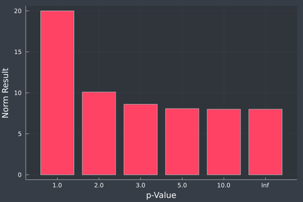
\[\eta(x) = \lVert \mathbf{x} \rVert_p = \Big( \sum_{i=1}^n \vert x_i \vert^p \Big)^{1/p}\,.\]

It's trivial to see that when \(p = 1\), we get the \(\ell^1\) norm, when \(p = 2\), we get the \(\ell^2\) norm, and so on. When \(p\) approaches \(\infty\), then we get the infinity norm which is defined as,

\[\eta(x) = \lVert \mathbf{x} \rVert_\infty = \max_i \vert x_i \vert \,.\]

l∞_norm(X) = [abs(x) for x in X] |> maximum

l∞_norm([4 ; 3])
> 4

Therefore, we can write a generalized function to handle any \(\ell^p\) norm as follows.

function lp_norm(X; p = 1)
    if isinf(p)
        [abs(x) for x in X] |> maximum
    else
        ([abs(x)^p for x in X] |> sum)^(1/p)
    end
end

@testset "ℓp Norms" begin
    X = [ 4 ; 3 ]
    @test lp_norm(X) == 7.0
    @test lp_norm(X; p=2) == 5.0
    @test lp_norm(X; p=Inf) == 4.0
end

>  Test Summary: | Pass  Total
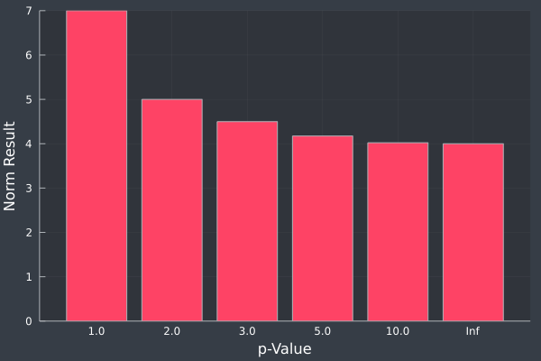
>  ℓp Norms      |    3      3

Interestingly, as \(p\) approaches \(\infty\), the result of \(\eta_p(x)\) approaches a minimum. The minimum here is, in fact, the maximum, unsigned component of \(\mathbf{x}\).

Looking at the \(p\) values of \(1\), \(2\), \(3\), \(5\), \(10\), and \(\infty\), for the \(2\)-dimensional vector, \((4, 3)\).

Plotting the same \(p\) values for a \(5\)-dimensional vector, \((4, 3, -2, 3, 8)\).