How To Analyze a Function
Suppose we want to analyze a function like,
\[ \Bigg( \frac{x + |x|}{2}\Bigg)^2 + \Bigg( \frac{x - |x|}{2}\Bigg)^2 = x^2\,, \]the first thing we'll usually do is try and get a sense of how the function behaves. This is essentially trying to get the "lay of the land." In fact, I usually use the term mapping instead of function as it's a much clearer word in my opinion and does a better job at representing what functions actually do.
The word function evokes a bit of a mechanical connotation, which is accurate enough in terms of it having an input and an output. It ellicits the vision of a machine where you plug in some value and it goes chug chug chug and some resulting value pops out. Thing is, we need to step back a bit and think about every possible value that could be plugged in and what do all of those points look like after our little function that could goes chug chug chug for a good, long while and spits out every possible result. More technically, this is called finding the domain and codomain of a mapping.
Getting back to \((1)\), we can see that \(x\) isn't constrained by any logarithms, trigonometric functions, or any non-elementary functions, so it looks like \(x\) can accept any rational numbers. How do we verify this? Back to the function mindset and we plug in some points to see what we get. This process is sped up quite a bit by simply plotting the function. A couple lines of Julia code later and voila!
function f(x)
    ((x + abs(x))/2)^2 + ((x - abs(x))/2)^2 - x^2
end

plot(f, ylim=(-1, 1), xlim=(-1000, 1000))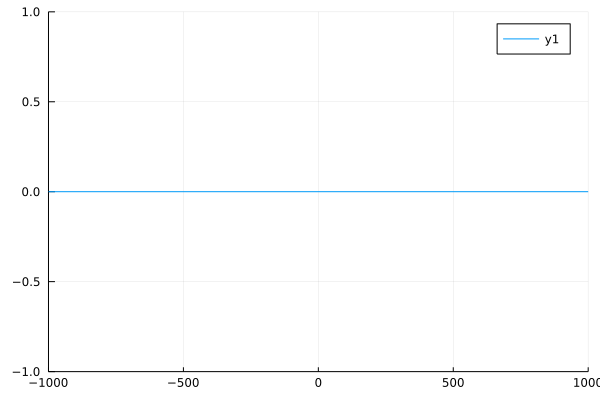
Such a simple plot offers some incredible insights into the function and helps steer our next steps. It appears that this equation is equivalent to the constant null function,
\[ f(x) = 0 \,.\]Examining \((1)\), we can see that the second term will always reduce to \(0\) and after simplifying the first term, the equation becomes,
\[ x^2 = x^2 \implies x^2 - x^2 = 0\,. \]Therefore, we have shown that \((1)\) maps all real values ranging from \(-\infty < x < \infty \) to \(0\). This means that \((1)\) is homomorphic to the constant null function, meaning they behave in the same way and have the same structure. With both functions, I can "plug in" any values in \(\mathbb{R}\) and will always get \(0\). Why have a specified values in \(\mathbb{R}\)? Because it turns out that when we plug in values from the complex numbers, \(\mathbb{C}\), we do not always get \(0\).
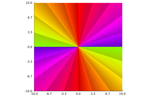
Using the ComplexPortraits package, we can visually see a phase plot of the function in the complex plane.
ComplexPortraits.phaseplot(-10.0 + 10.0im, 10.0 - 10.0im, z -> f(z))